Lolly's Final Report
Introduction
Pattern recognition is machine learning. It focuses on the recognition of patterns and regularities in data. Pattern recognition makes inferences from perceptual data, and it uses tools from statistics, probability, computational geometry, machine learning, signal processing, and algorithm design. Pattern recognition can recognize patterns.
From automated speech recognition, fingerprint identification, optical character recognition, DNA sequence identification. It is importance to artificial intelligence and computer vision, and has far-reaching applications in engineering, science, medicine, and business.
If the characteristics or attributes of a class are known, individual objects might be identified as belonging or not belonging to that class. The objects are assigned to classes by observing patterns of distinguishing characteristics and comparing them to a model member of each class.
Pattern recognition is categorized according to the type of learning procedure used to generate the output value. Supervised learning assumes that a training data has been provided, consisting of a set of instances that have been properly labeled by hand with the correct output. Perform as well as possible on the training data, and generalize as well as possible to new data. Unsupervised learning assumes training data that has not been hand-labeled, and attempts to find inherent patterns in the data that can be used to determine the correct output value for new data instances. A combination of the two that has recently been explored is semi-supervised learning, which uses a combination of labeled and unlabeled data. In unsupervised learning, there may be no training data at all to speak of, in other words, the data to be labeled is the training data. Sometimes different terms are used to describe the corresponding supervised and unsupervised learning procedures for the same type of output.
Pattern recognition involves the extraction of patterns from data, their analysis and, finally, the identification of the category each of the pattern belongs to. A typical pattern recognition system contains a sensor, a preprocessing mechanism, a feature extraction mechanism, a classification or description algorithm, and a set of examples already classified or described.
A neural network is a powerful computational data model that is able to capture and represent complex input and output relationships. The motivation for the development of neural network technology supported from the desire to develop an artificial system that could perform "intelligent" tasks similar to those performed by the human brain.
The true power and advantage of neural networks lies in their ability to represent both linear and non-linear relationships and in their ability to learn these relationships directly from the data being modeled. Traditional linear models are simply unsatisfactory when it comes to modeling data that contains non-linear characteristics.
The most common neural network model is the Multilayer Perceptron (MLP). This type of neural network is known as a supervised network because it requires a desired output in order to learn. The goal of this type of network is to create a model that correctly maps the input to the output using historical data so that the model can then be used to produce the output when the desired output is unknown.
The MLP and many other neural networks learn using an algorithm called backpropagation. With backpropagation, the input data is repeatedly presented to the neural network. With each presentation the output of the neural network is compared to the desired output and an error is computed. This error is then fed back (backpropagate) to the neural network and used to adjust the weights such that the error decreases with each iteration and the neural model gets closer and closer to producing the desired output. This process is known as "training".
Neural networks are organized in layers. Layers are made up of a number of interconnected 'nodes' which contain an 'activation function'. Patterns are presented to the network by the way of the 'input layer', which communicates to one or more 'hidden layers' where the actual processing is done by a system of weighted 'connections'.
What is deep neural networks, meaning ones in which we have multiple hidden layers. It is common to have neural networks with more than 10 layers and even more than 100 layer ANNs are tried. This will allow us to compute much more complex features of the input. Because each hidden layer computes a non-linear transformation of the previous layer, a deep network can have significantly greater representational power than a shallow one.
When training a deep network, it is important to use a non-linear activation function in each hidden layer. This is because multiple layers of linear functions would itself compute only a linear function of the input, and thus be no more expressive than using just a single layer of hidden units.
You can essentially stack layers of neurons on top of each other. The lowest layer takes the raw data like images, text, sound, etc. and then each neurons stores some information about the data. Each neuron in the layer sends information up to the next layers of neurons which learn a more abstract version of the data. So the higher you go up, the more abstract features you learn.
Deep learning refers to neural nets with more than one hidden layer. The depth of the neural net allows it to construct a feature hierarchy of increasing abstraction, with each subsequent layer acting as a filter for more and more complex features that combine those of the previous layer. This feature hierarchy and the filters which model significance in the data, is created automatically when deep nets learn to reconstruct unsupervised data. Because they can work with unsupervised data, which constitutes the majority of data in the world, deep nets can become more accurate than traditional multilayer algorithms that are unable to handle unsupervised data. That is, the algorithms with access to more data win. Why neural network and deep neural network can be used in pattern recognition? Because they can remember what is true and what is false, and can learning. After learning, they can correctly recognize the pattern.
Reading content
Decision tree has many dimensions. Dimensions in a data set are called features, predictors, or variables. Adding another dimension allows for more nuance. When we build the tree, a decision tree has to get the first feature, which is called the node in the training data. What the feature does the decision tree select? A decision tree can find the better feature by itself. In machine learning, these statements are called Forks, and they split the data into two branches based on some value. Repeat this method again and again. This repetition is called Recursion. The more forks you add, the more prediction accuracy. These ultimate branches of the tree are called Leaf Nodes. The tree’s predictions are 100% accurate, because it was used to train the model, this data is called training data. To test the tree’s performance on new data, we need to apply it to data points that it has never seen before. This previously unused data is called test data. The tree should perform similarly on training data and test data.
Random Forest is built by many Decision Tree. These tree are combined by different data and features, and the conclusion will be different. This method is called Bagging. If every trees use different features and data, it will be have a problem. The problem is some trees have many nodes, some trees have a few nodes, some trees are wide, and some trees are skew. Therefore, we should give the suitable amount of feature to the trees. Finally, Random Forest uses method of Ensemble to combine all of tree. After the Random forest was built, we put data into the random forest. We probably have a rate of mistake. This is called Out-Of-Bag.
A Multilayer Perceptron (MLP) is a type of neural network referred to as a supervised network because it requires a desired output in order to learn. The goal of this type of network is to create a model that correctly maps the input to the output using pre-chosen data so that the model can then be used to produce the output when the desired output is unknown. The MLP learns using an algorithm called backpropagation. With backpropagation, the input data is repeatedly presented to the neural network in a process known as "training". With each presentation the output of the neural network is compared to the desired output and an error is computed. This error is then fed back to the neural network and used to adjust the weights such that the error decreases with each iteration and the neural model gets closer and closer to producing the desired output.
Fed forward neural networks is mean that there are no loops in the network, information is always fedforward, never feedback.
Sigmoid neurons are similar to perceptrons, but modified that small changes in their weights and bias cause only a small change in their output. While sigmoid neurons have much of the same qualitative behaviour as perceptrons, they make it much easier to figure out how changing the weights and biases will change the output. One big difference between perceptrons and sigmoid neurons is that sigmoid neurons don't just output 0 or 1. They can have as output any real number between 0 and 1.
A perceptron takes several binary inputs, and produces a single binary output. The neuron's output, 0 or 1, is determined by whether the weighted sum is less than or greater than some threshold value. By varying the weights and the threshold, we can get different models of decision-making.
Perceptron can be used is to compute the elementary logical functions we usually think of as underlying computation, functions such as AND, OR, and NAND.
Using the method of cross-entropy cost function, we'll suppose instead that we're trying to train a neuron with several input variables, corresponding weights and a bias. The output from the neuron is a=, is the weighted sum of the inputs. Two properties interpret the cross-entropy as a cost function. First, it's non-negative. Second, if the neuron's actual output is close to the desired output for all training inputs, then the cross-entropy will be close to zero.
Universality theorem holds even if we limit our networks to have just a single layer between the input and the output neurons single hidden layer. So even very simple network architectures can be extremely powerful. By increasing the number of hidden neurons we can improve the approximation. Continuous functions, if a function is discontinuous, then it won't be possible to approximate using a neural net. A more precise statement of the universality theorem is that neural networks with a single hidden layer can be used to approximate any continuous function to any desired precision
We learned that deep neural networks are often much harder to train. If we could train deep nets they should be much more powerful. Connect the input pixels to a layer of hidden neurons. But we won't connect every input pixel to every hidden neuron. Instead, we only make connections in small, localized regions of the input image. Building up the first hidden layer. If we have a 28×28 input image, this means our network has 784 (28×28) input neurons, and 5×5 local receptive fields, then there will be 24×24 neurons in the hidden layer. This is because we can only move the local receptive field 23 neurons across. This means that all the neurons in the first hidden layer detect the same feature, just at different location in the input image. To see why this makes sense, suppose the weights and bias are such that the hidden neuron can pick out. So a complete convolutional layer consists of several different feature maps. To do image recognition we'll need more than one feature map.
Pooling layers are usually used immediately after convolutional layers. What the pooling layers do is simplify the information in the output from the convolutional layer. In detail, a pooling layer takes each feature map output from the convolutional layer and prepares a condensed feature map. To use training data to train the network's weights and biases so that the network does a good job classifying input digits.
What is Recurrent Neural Networks (RNNs), Long Short-Term Memory Networks (LSTMs), and Deep Belief Nets. Recurrent Neural Networks (RNNs) connect output to the input, it can return the last time of output and record in the neurons, this Neural Network is similar to the latch. Recurrent Neural Network let the last time of output relate to the next time of input. That’s mean the Recurrent Neural Network have correlation and have memory.
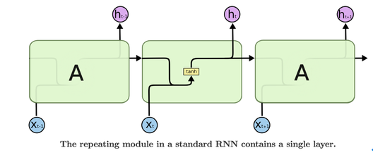
Long Short-Term Memory Networks (LSTMs) are a special kind of RNN. All recurrent neural networks have the form of repeating modules of neural network. In standard RNNs, this repeating module will have a very simple structure, such as a single tanh layer.
Pattern recognition is machine learning. It focuses on the recognition of patterns and regularities in data. Pattern recognition makes inferences from perceptual data, and it uses tools from statistics, probability, computational geometry, machine learning, signal processing, and algorithm design. Pattern recognition can recognize patterns.
From automated speech recognition, fingerprint identification, optical character recognition, DNA sequence identification. It is importance to artificial intelligence and computer vision, and has far-reaching applications in engineering, science, medicine, and business.
If the characteristics or attributes of a class are known, individual objects might be identified as belonging or not belonging to that class. The objects are assigned to classes by observing patterns of distinguishing characteristics and comparing them to a model member of each class.
Pattern recognition is categorized according to the type of learning procedure used to generate the output value. Supervised learning assumes that a training data has been provided, consisting of a set of instances that have been properly labeled by hand with the correct output. Perform as well as possible on the training data, and generalize as well as possible to new data. Unsupervised learning assumes training data that has not been hand-labeled, and attempts to find inherent patterns in the data that can be used to determine the correct output value for new data instances. A combination of the two that has recently been explored is semi-supervised learning, which uses a combination of labeled and unlabeled data. In unsupervised learning, there may be no training data at all to speak of, in other words, the data to be labeled is the training data. Sometimes different terms are used to describe the corresponding supervised and unsupervised learning procedures for the same type of output.
Pattern recognition involves the extraction of patterns from data, their analysis and, finally, the identification of the category each of the pattern belongs to. A typical pattern recognition system contains a sensor, a preprocessing mechanism, a feature extraction mechanism, a classification or description algorithm, and a set of examples already classified or described.
A neural network is a powerful computational data model that is able to capture and represent complex input and output relationships. The motivation for the development of neural network technology supported from the desire to develop an artificial system that could perform "intelligent" tasks similar to those performed by the human brain.
The true power and advantage of neural networks lies in their ability to represent both linear and non-linear relationships and in their ability to learn these relationships directly from the data being modeled. Traditional linear models are simply unsatisfactory when it comes to modeling data that contains non-linear characteristics.
The most common neural network model is the Multilayer Perceptron (MLP). This type of neural network is known as a supervised network because it requires a desired output in order to learn. The goal of this type of network is to create a model that correctly maps the input to the output using historical data so that the model can then be used to produce the output when the desired output is unknown.
The MLP and many other neural networks learn using an algorithm called backpropagation. With backpropagation, the input data is repeatedly presented to the neural network. With each presentation the output of the neural network is compared to the desired output and an error is computed. This error is then fed back (backpropagate) to the neural network and used to adjust the weights such that the error decreases with each iteration and the neural model gets closer and closer to producing the desired output. This process is known as "training".
Neural networks are organized in layers. Layers are made up of a number of interconnected 'nodes' which contain an 'activation function'. Patterns are presented to the network by the way of the 'input layer', which communicates to one or more 'hidden layers' where the actual processing is done by a system of weighted 'connections'.
What is deep neural networks, meaning ones in which we have multiple hidden layers. It is common to have neural networks with more than 10 layers and even more than 100 layer ANNs are tried. This will allow us to compute much more complex features of the input. Because each hidden layer computes a non-linear transformation of the previous layer, a deep network can have significantly greater representational power than a shallow one.
When training a deep network, it is important to use a non-linear activation function in each hidden layer. This is because multiple layers of linear functions would itself compute only a linear function of the input, and thus be no more expressive than using just a single layer of hidden units.
You can essentially stack layers of neurons on top of each other. The lowest layer takes the raw data like images, text, sound, etc. and then each neurons stores some information about the data. Each neuron in the layer sends information up to the next layers of neurons which learn a more abstract version of the data. So the higher you go up, the more abstract features you learn.
Deep learning refers to neural nets with more than one hidden layer. The depth of the neural net allows it to construct a feature hierarchy of increasing abstraction, with each subsequent layer acting as a filter for more and more complex features that combine those of the previous layer. This feature hierarchy and the filters which model significance in the data, is created automatically when deep nets learn to reconstruct unsupervised data. Because they can work with unsupervised data, which constitutes the majority of data in the world, deep nets can become more accurate than traditional multilayer algorithms that are unable to handle unsupervised data. That is, the algorithms with access to more data win. Why neural network and deep neural network can be used in pattern recognition? Because they can remember what is true and what is false, and can learning. After learning, they can correctly recognize the pattern.
Reading content
Decision tree has many dimensions. Dimensions in a data set are called features, predictors, or variables. Adding another dimension allows for more nuance. When we build the tree, a decision tree has to get the first feature, which is called the node in the training data. What the feature does the decision tree select? A decision tree can find the better feature by itself. In machine learning, these statements are called Forks, and they split the data into two branches based on some value. Repeat this method again and again. This repetition is called Recursion. The more forks you add, the more prediction accuracy. These ultimate branches of the tree are called Leaf Nodes. The tree’s predictions are 100% accurate, because it was used to train the model, this data is called training data. To test the tree’s performance on new data, we need to apply it to data points that it has never seen before. This previously unused data is called test data. The tree should perform similarly on training data and test data.
Random Forest is built by many Decision Tree. These tree are combined by different data and features, and the conclusion will be different. This method is called Bagging. If every trees use different features and data, it will be have a problem. The problem is some trees have many nodes, some trees have a few nodes, some trees are wide, and some trees are skew. Therefore, we should give the suitable amount of feature to the trees. Finally, Random Forest uses method of Ensemble to combine all of tree. After the Random forest was built, we put data into the random forest. We probably have a rate of mistake. This is called Out-Of-Bag.
A Multilayer Perceptron (MLP) is a type of neural network referred to as a supervised network because it requires a desired output in order to learn. The goal of this type of network is to create a model that correctly maps the input to the output using pre-chosen data so that the model can then be used to produce the output when the desired output is unknown. The MLP learns using an algorithm called backpropagation. With backpropagation, the input data is repeatedly presented to the neural network in a process known as "training". With each presentation the output of the neural network is compared to the desired output and an error is computed. This error is then fed back to the neural network and used to adjust the weights such that the error decreases with each iteration and the neural model gets closer and closer to producing the desired output.
Fed forward neural networks is mean that there are no loops in the network, information is always fedforward, never feedback.
Sigmoid neurons are similar to perceptrons, but modified that small changes in their weights and bias cause only a small change in their output. While sigmoid neurons have much of the same qualitative behaviour as perceptrons, they make it much easier to figure out how changing the weights and biases will change the output. One big difference between perceptrons and sigmoid neurons is that sigmoid neurons don't just output 0 or 1. They can have as output any real number between 0 and 1.
A perceptron takes several binary inputs, and produces a single binary output. The neuron's output, 0 or 1, is determined by whether the weighted sum is less than or greater than some threshold value. By varying the weights and the threshold, we can get different models of decision-making.
Perceptron can be used is to compute the elementary logical functions we usually think of as underlying computation, functions such as AND, OR, and NAND.
Using the method of cross-entropy cost function, we'll suppose instead that we're trying to train a neuron with several input variables, corresponding weights and a bias. The output from the neuron is a=, is the weighted sum of the inputs. Two properties interpret the cross-entropy as a cost function. First, it's non-negative. Second, if the neuron's actual output is close to the desired output for all training inputs, then the cross-entropy will be close to zero.
Universality theorem holds even if we limit our networks to have just a single layer between the input and the output neurons single hidden layer. So even very simple network architectures can be extremely powerful. By increasing the number of hidden neurons we can improve the approximation. Continuous functions, if a function is discontinuous, then it won't be possible to approximate using a neural net. A more precise statement of the universality theorem is that neural networks with a single hidden layer can be used to approximate any continuous function to any desired precision
We learned that deep neural networks are often much harder to train. If we could train deep nets they should be much more powerful. Connect the input pixels to a layer of hidden neurons. But we won't connect every input pixel to every hidden neuron. Instead, we only make connections in small, localized regions of the input image. Building up the first hidden layer. If we have a 28×28 input image, this means our network has 784 (28×28) input neurons, and 5×5 local receptive fields, then there will be 24×24 neurons in the hidden layer. This is because we can only move the local receptive field 23 neurons across. This means that all the neurons in the first hidden layer detect the same feature, just at different location in the input image. To see why this makes sense, suppose the weights and bias are such that the hidden neuron can pick out. So a complete convolutional layer consists of several different feature maps. To do image recognition we'll need more than one feature map.
Pooling layers are usually used immediately after convolutional layers. What the pooling layers do is simplify the information in the output from the convolutional layer. In detail, a pooling layer takes each feature map output from the convolutional layer and prepares a condensed feature map. To use training data to train the network's weights and biases so that the network does a good job classifying input digits.
What is Recurrent Neural Networks (RNNs), Long Short-Term Memory Networks (LSTMs), and Deep Belief Nets. Recurrent Neural Networks (RNNs) connect output to the input, it can return the last time of output and record in the neurons, this Neural Network is similar to the latch. Recurrent Neural Network let the last time of output relate to the next time of input. That’s mean the Recurrent Neural Network have correlation and have memory.
Long Short-Term Memory Networks (LSTMs) are a special kind of RNN. All recurrent neural networks have the form of repeating modules of neural network. In standard RNNs, this repeating module will have a very simple structure, such as a single tanh layer.
Long Short-Term Memory Networks are explicitly designed to avoid the long-term dependency problem. Long Short-Term Memory Networks also have this chain like structure, but the repeating module has a different structure. Instead of having a single neural network layer, there are four, interacting in a very special way.
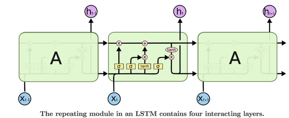
The sigmoid layer outputs numbers between zero and one, describing how much of each component should be let through. A value of zero means “let nothing through,” while a value of one means “let everything through”. An LSTM has three of these gates, to protect and control the cell state. The first step in our LSTM is to decide what information we’re going to throw away from the cell state. This decision is made by a sigmoid layer called the “forget gate layer.”
The second step is to decide what new information we’re going to store in the cell state. This has two parts. First, a sigmoid layer called the “input gate layer” decides which values we’ll update. Second, a tan(h) layer creates a vector of new candidate values.
Finally, we need to decide what we’re going to output. First, we run a sigmoid layer which decides what parts of the cell state we’re going to output. Then, we put the cell state through tan(h) (to push the values to be between −1 and 1) and multiply it by the output of the sigmoid gate, so that we get the output This output will be based on our cell state, but will be a filtered version.
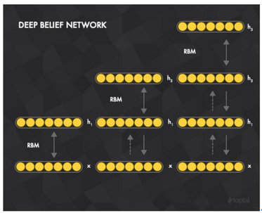
The deep belief nets training method is called a fast, greedy algorithm. We believe that the composition of x and h1 RBM, its training. After fixing w, training h1 and h2, and so on.
The second step is to decide what new information we’re going to store in the cell state. This has two parts. First, a sigmoid layer called the “input gate layer” decides which values we’ll update. Second, a tan(h) layer creates a vector of new candidate values.
Finally, we need to decide what we’re going to output. First, we run a sigmoid layer which decides what parts of the cell state we’re going to output. Then, we put the cell state through tan(h) (to push the values to be between −1 and 1) and multiply it by the output of the sigmoid gate, so that we get the output This output will be based on our cell state, but will be a filtered version.
The deep belief nets training method is called a fast, greedy algorithm. We believe that the composition of x and h1 RBM, its training. After fixing w, training h1 and h2, and so on.
Learning from group discussion
Gradient Descent (GD) also call greedy algorithm. It just find the valley. Stochastic Gradient Descent (SGD) can find the real zero, and Stochastic Gradient Descent is faster than Gradient Descent. Stochastic Gradient Descent is fast to find valley, but its’ accuracy is slow. Using mini-batch, Stochastic Gradient Descent to increase the accuracy. Stochastic Gradient Descent is faster than mini-batch and Gradient Descent in the learning speed. Gradient Descent is more accurate than mini-batch and Stochastic Gradient Descent.
The backpropagation calculate the weight from final layer to first layer. In backpropagation, first, we have the input through the network and get the output and the cost function of output. After that, we can get the cost function in each layer, and we will use the gradient descent to calculate the update weight in each layer.
In the traditional neural network, the more neurons in the hidden layer, the more errors will be. Because conclusion of all neurons are not really correct, many neurons are not the good way. Using dropout can decrease the neurons. All neurons in the network can’t see all the data. After training another neurons will come back to input and training data again. Thus, the accuracy will be better than the traditional neural network.
Except for step function, other activation functions with two properties. First property is assume s(z) is well-defined as z- and z. Second property, we need to assume that these limits are different from one another. These two properties can also help neural networks achieve function approximation.
There are four factors that make the training of Deep Neural Networks hard to train. First is instability of gradients, that’s mean, the next of layer is faster than the previous of layer, and the vanishing gradient problem occurs. It is difficult to training Deep Neural Networks. Second, because we use sigmoid function, we will have the vanishing gradient problem. We choice the activation function to training Deep Neural Networks. Third, if we use the way weights are initialized, training Deep Neural Networks will be saturation and be slow. Fourth, hyper-parameters include regularization section and learning rate. If learning rate is small, learning will be slow. If learning rate is large, learning will be overshot.
There are seven versions of Neural Network/Deep. Neural Network for MNIST with improved accuracy from 97.8% to 99.6%. Each version adds one more technique to the learning algorithm of previous version. First, we’ll start with a shallow architecture, just one hidden layer. Accuracy is 97.8%. Second, using Deep network, convolutional layer, pooling layer and fully-connected layer. Accuracy is 98.78%.
Third, using Deep network, convolutional layer, pooling layer, second convolutional pooling layer and fully-connected layer. Accuracy is 99.06%. Fourth, using rectified linear units instead of using a sigmoid activation function. Accuracy is 99.23%. Fifth, expanding the training data. Accuracy is 99.37%. Sixth, inserting an extra fully-connected layer. Accuracy is 99.43%. Seventh, applying dropout. Accuracy is 99.6%.
Conclusion
I’m so happy to choose this class and I like the form of this course. This course is not like the other general courses. The other courses are regularization. After this class, I understood many about technology and knowledge of pattern recognition. I knew the application of pattern recognition and how practical and powerful is it. I got great benefits in this course. I believe this technology will be very popular and formidable in the future.
