Tommy's Final Report
Introduction
1. What is pattern recognition
(1) Fundamental concepts of PR
Feature can be defined as any distinctive aspect, quality or characteristic which, may be symbolic or numeric. The combination of features is represented as a d-dimensional column vector called a feature vector. The d-dimensional space defined by the feature vector is called feature space. Objects are represented as points in feature space. This representation is called a scatter plot.
Pattern is defined as composite of features that are characteristic of an individual. In classification, a pattern is a pair of variables {x,w} where x is a collection of observations or features and w is the concept behind the observation. The quality of a feature vector is related to its ability to discriminate examples from different classes . Examples from the same class should have similar feature values and while examples from different classes having different feature values.
(2) Steps or algorithms of PR
Pattern recognition involves the extraction of patterns from data, their analysis and, finally, the identification of the category each of the pattern belongs to. A typical pattern recognition system contains a sensor, a preprocessing mechanism, a feature extraction mechanism (manual or automated), a classification or description algorithm, and a set of examples (training set) already classified or described
(3) Applications of PR
To illustrate the complexity of some of the types of problems involved, consider the following example. Suppose that a fish-packing plant wants to automate the process of sorting incoming fish on a conveyor belt according to species. As a pilot project, it is decided to try to separate sea bass from salmon using optical sensing.
Set up a camera, take some sample images, and begin to note some physical differences between the two types of fish, length, lightness, width, number and shape of fins, position of the mouth, and so on, and these suggest features to explore for use in our classifier.
(4) Goal of PR
Pattern recognition is the science of making inferences from perceptual data, using tools from statistics, probability, computational geometry, machine learning, signal processing, and algorithm design. Thus, it is of central importance to artificial intelligence and computer vision, and has far-reaching applications in engineering, science, medicine, and business. In particular, advances made during the last half century, now allow computers to interact more effectively with humans and the natural world. However, the most important problems in pattern recognition are yet to be solved.
2. Neural Networks and Deep Neural Networks
(1) What is NN/DNN
In machine learning and cognitive science, neural networks (NNs) are a family of models inspired by biological neural networks (the central nervous systems of animals, in particular the brain) which are used to estimate or approximate functions that can depend on a large number of inputs and are generally unknown. Artificial neural networks are typically specified using three things:
Architecture: specifies what variables are involved in the network and their topological relationships—for example the variables involved in a neural network might be the weights of the connections between the neurons, along with activities of the neurons.
Activity Rule: Most neural network models have short time-scale dynamics: local rules define how the activities of the neurons change in response to each other. Typically the activity rule depends on the weights in the network.
Learning Rule: The learning rule specifies the way in which the neural network's weights change with time. This learning is usually viewed as taking place on a longer time scale than the time scale of the dynamics under the activity rule. Usually the learning rule will depend on the activities of the neurons. It may also depend on the values of the target values supplied by a teacher and on the current value of the weights.
For example, a neural network for handwriting recognition is defined by a set of input neurons which may be activated by the pixels of an input image. After being weighted and transformed by a function, the activations of these neurons are then passed on to other neurons. This process is repeated until finally, the output neuron that determines which character was read is activated.
Like other machine learning methods – systems that learn from data – neural networks have been used to solve a wide variety of tasks, like computer vision and speech recognition, that are hard to solve using ordinary rule-based programming.
(2) Why NN/DNN can be a good PR method
Neural networks are similar to biological neural networks in the performing by its units of functions collectively and in parallel, rather than by a clear delineation of subtasks to which individual units are assigned. The term "neural network" usually refers to models employed in statistics, cognitive psychology and artificial intelligence. Neural network models which command the central nervous system and the rest of the brain are part of theoretical neuroscience and computational neuroscience.
In modern software implementations of artificial neural networks, the approach inspired by biology has been largely abandoned for a more practical approach based on statistics and signal processing. In some of these systems, neural networks or parts of neural networks form components in larger systems that combine both adaptive and non-adaptive elements. While the more general approach of such systems is more suitable for real-world problem solving, it has little to do with the traditional, artificial intelligence connectionist models. What they do have in common, however, is the principle of non-linear, distributed, parallel and local processing and adaptation. Historically, the use of neural network models marked a directional shift in the late eighties from high-level artificial intelligence, characterized by expert systems with knowledge embodied in if-then rules, to low-level machine learning, characterized by knowledge embodied in the parameters of a dynamical system.
Reading contents
1. Linear classifier and neural networks
(1) Basic definition of linear classifier
In the field of machine learning, the goal of statistical classification is to use an object's characteristics to identify which class (or group) it belongs to. A linear classifier achieves this by making a classification decision based on the value of a linear combination of the characteristics. An object's characteristics are also known as feature values and are typically presented to the machine in a vector called a feature vector.
If the input feature vector to the classifier is a real vector x , then the output score is
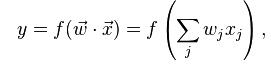
where vector w is a real vector of weights and f is a function that converts the dot product of the two vectors into the desired output. The weight vector w is learned from a set of labeled training samples. Often f is a simple function that maps all values above a certain threshold to the first class and all other values to the second class.
(2) Geometric interpretation of linear classifier
The geometrical interpretation depicted may help its to better understand the function of a single neuron. The n input values of a neuron may be interpreted as coordinates of a point in the n-dimensional Euclidean input space.
(3) Perceptron
In machine learning, the perceptron is an algorithm for supervised learning of binary classifiers: functions that can decide whether an input (represented by a vector of numbers) belongs to one class or another. It is a type of linear classifier, i.e. a classification algorithm that makes its predictions based on a linear predictor function combining a set of weights with the feature vector. The algorithm allows for online learning, in that it processes elements in the training set one at a time.
(4) Relation of linear classifier and perceptron
The perceptron is a linear classifier, therefore it will never get to the state with all the input vectors classified correctly if the training set D is not linearly separable, i.e. if the positive examples can not be separated from the negative examples by a hyperplane. In this case, no "approximate" solution will be gradually approached under the standard learning algorithm, but instead learning will fail completely. Hence, if linear separability of the training set is not known a priori, one of the training variants below should be used.
But if the training set is linearly separable, then the perceptron is guaranteed to converge, and there is an upper bound on the number of times the perceptron will adjust its weights during the training.
2. How does machine learning work: decision tree as an example
(1) Decision tree
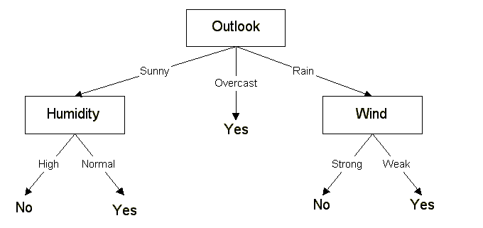
Decision tree represents a mapping between objects and object attributes values. Each node in the tree mean an object, and every path are represent a possible attribute value, and each leaf node objects corresponding value which is from root to the leaf node. Decision tree only a single output. If we want have a complex output, we can build an independent decision tree to handle different output (as figure 1).
(2) Geometric interpretation of linear classifier
The geometrical interpretation depicted may help its to better understand the function of a single neuron. The n input values of a neuron may be interpreted as coordinates of a point in the n-dimensional Euclidean input space.
(3) Perceptron
In machine learning, the perceptron is an algorithm for supervised learning of binary classifiers: functions that can decide whether an input (represented by a vector of numbers) belongs to one class or another. It is a type of linear classifier, i.e. a classification algorithm that makes its predictions based on a linear predictor function combining a set of weights with the feature vector. The algorithm allows for online learning, in that it processes elements in the training set one at a time.
(4) Relation of linear classifier and perceptron
The perceptron is a linear classifier, therefore it will never get to the state with all the input vectors classified correctly if the training set D is not linearly separable, i.e. if the positive examples can not be separated from the negative examples by a hyperplane. In this case, no "approximate" solution will be gradually approached under the standard learning algorithm, but instead learning will fail completely. Hence, if linear separability of the training set is not known a priori, one of the training variants below should be used.
But if the training set is linearly separable, then the perceptron is guaranteed to converge, and there is an upper bound on the number of times the perceptron will adjust its weights during the training.
2. How does machine learning work: decision tree as an example
(1) Decision tree
Decision tree represents a mapping between objects and object attributes values. Each node in the tree mean an object, and every path are represent a possible attribute value, and each leaf node objects corresponding value which is from root to the leaf node. Decision tree only a single output. If we want have a complex output, we can build an independent decision tree to handle different output (as figure 1).
Data Mining Decision Tree is a regular use of the technology can be used to analyze the data, also can be used to make predictions. Decision is a common method in data mining. In the data mining, every decision tree mean the tree structure, it the type of follow branches to classify. Each tree can rely on the divided source for data testing. The process can be recursive pruning. When it doesn't be separating division or class can be applied to a branch, the recursive is complete.
(2) Decision forest
In a machine learning, decision forest is a classifier including lots of Decision tree, and its output category is by individual tree to produce.
(3) The relationship between decision tree and random forest
Random forests is a idea of random decision forests that are a learning method for classification, regression and other tasks, that operate by constructing a multitude of decision trees at training time and outputting the class that is the mode of the classification or mean prediction (regression) of the individual trees.
According to the following to build every tree:
I. Use N number to represent training case, M mean number of features.
II. Input feature number m, which is used to determine the results of the decision tree node(m should be less than M).
III. From N training samples to sampling with replacement mode, sampling N times to form a training set and not be able to get samples for use to anticipate, evaluate the error.
IV. For each node, chose m feature randomly, decided that each node on the tree are determined base on these characteristics , according to these features to calculate the best way to split.
(4) ID3(Iterative Dichotomiser 3) algorithm example
ID3 algorithm Gain values for each property and select the highest gain property to property as a test set. Create a node is selected for testing properties, and the properties of the node is created for each branch and by this attribute to calculate the other samples. Gain measure how well given attribute separates training examples into targeted classes. In order to define gain, It has an idea from information theory called entropy.
Given a collection S of outcomes
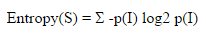
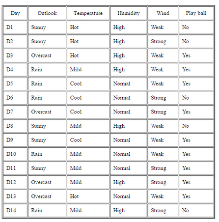
Example 1: if S is a collection of 14 examples with 9 YES and 5 NO examples then
Entropy(S)= - (9/14) log2 (9/14) - (5/14) log2 (5/14) = 0.940
Entropy is 0 if member of S belong to the same class, The range of entropy is 0 to 1
Gain(S, A) is information gain of example set S on attribute A is defined as
Gain(S, A) = Entropy(S) -total attribute[ ((|Sv| / |S|) * Entropy(Sv)) ]
Example 2: suppose S is a set of 14 examples in which one of attributes is wind speed. In the 14 examples are 9 YES and 5 NO. If only see attribute wind, 8 occurrences of weak wind and 6 occurrences of strong wind. For wind is weak, 6 of examples are YES and 2 are NO, for wind is strong, 3 of examples are YES and 3 are NO.
so that
Gain(S,Wind)=Entropy(S)-(8/14)*Entropy(Sweak)-(6/14)*Entropy(Sstrong)
=0.940 - (8/14)*0.811 - (6/14)*1.00 =0.048
which
Entropy(Sweak) = - (6/8)*log2(6/8) - (2/8)*log2(2/8) = 0.811
Entropy(Sstrong) = - (3/6)*log2(3/6) - (3/6)*log2(3/6) = 1.00
|
Gain(S, Outlook) = 0.246
Gain(S, Temperature) = 0.029 Gain(S, Humidity) = 0.151 Gain(S, Wind) = 0.048 Outlook attribute has the highest gain, so it used as the root node. Ssunny = {D1, D2, D8, D9, D11} = 5 examples from table 1 with outlook = sunny Gain(Ssunny, Humidity) = 0.970 Gain(Ssunny, Temperature) = 0.570 Gain(Ssunny, Wind) = 0.019 |
3. Perceptron learning algorithm
(1) What is perceptron by representing it with the formula of linear classifiers
In machine learning, perception is supervised binary classification learning algorithm. Function can determine an input belong to a class or the other linear classification, also named the classification algorithm, making based on a linear predictor function a set of weights and a combination of feature vectors forecast.The algorithm allows for online learning, in that it processes elements in the training set one at a time.
(2) The learning algorithm of perceptron.
Multilayer Perceptron is an example of a perceptual learning algorithm. Multilayer Perceptron, which, in the presence of a hidden layer, you must use a more complex algorithm, such as back-propagation. Alternatively, the method may be as delta rule if the function is non-linear and differentiable, although a work in the following and use.
When multiple-aware artificial neural networks, each output neuron independent of all other work; therefore, learning each output can be considered separately.
(3) Formula of the delta rule
In machine learning, the delta rule is a gradient descent learning rule for updating the weights of the inputs to artificial neurons in a single-layer neural network.
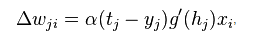
where
Alpha is a small constant called learning rate
g(x) is the neuron's activation function
tj is the target output
hj is the weighted sum of the neuron's inputs
yj is the actual output
xi is the the input.
The delta rule is commonly stated in simplified form for a neuron with a linear activation function as
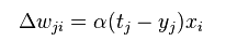
The delta rule is similar to the perception update rules, and the derivation is different. Perception using the unit step function as the activation function g(h), and this means g'(h) at zero does not exist elsewhere and is equal to zero, which makes the direct application of the delta rule impossible.
4. MLP and XOR
(1) What is MLP
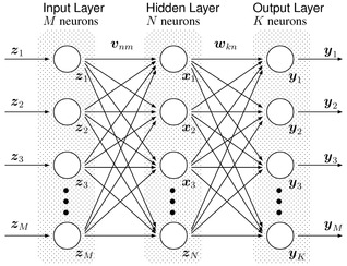
Multilayer Perceptron (MLP) is a forward structure of artificial neural network, which is mapping a set of input vectors to output vectors.
MLP can be viewed as a directed graph consists of nodes composed of multiple layers, each layer is fully connected to the next layer. Except the input node, each node is a neuron non-linear activation function. Supervised learning method called back propagation algorithm is often used to train the MLP. MLP is the perception of the promotion, we can not overcome the perception of non-linear partial data to identify weaknesses.
Multilayer perceptrons also using in backpropagation algorithm which is the standard algorithm for any supervised learning pattern recognition process and the subject of ongoing research in computational neuroscience and parallel distributed processing. They are useful in research in terms of their ability to solve problems stochastically, which often allows one to get approximate solutions for extremely complex problems like fitness approximation.
4. MLP and XOR
(1) What is MLP
Multilayer Perceptron (MLP) is a forward structure of artificial neural network, which is mapping a set of input vectors to output vectors.
MLP can be viewed as a directed graph consists of nodes composed of multiple layers, each layer is fully connected to the next layer. Except the input node, each node is a neuron non-linear activation function. Supervised learning method called back propagation algorithm is often used to train the MLP. MLP is the perception of the promotion, we can not overcome the perception of non-linear partial data to identify weaknesses.
Multilayer perceptrons also using in backpropagation algorithm which is the standard algorithm for any supervised learning pattern recognition process and the subject of ongoing research in computational neuroscience and parallel distributed processing. They are useful in research in terms of their ability to solve problems stochastically, which often allows one to get approximate solutions for extremely complex problems like fitness approximation.
(2) Difference between Perceptron and MLP
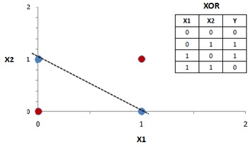
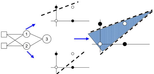
The main difference between Perceptron and MLP is the number of layers. A Perceptorn only have single layers and it can only solve problem with linear function. Single perception are quite limited, for example, see the famous XOR problem, which is separating hyperplane can not be used. Compared to single-layer perceptron, MLP is the standard perception of a single layer is deformed and can not belong to distinguish linearly separable data, to overcome the perceived weakness monolayer.
(3) Why MLP can solve XOR
Below figure mean single layer perceptron can't solve the XOR problem, because which is not linearly separable. MLP is difference with single layerperceptorn, so that it can solve the XOR problem.
|
|
5. Backpropagation learning algorithm
(1) Why use sigmoid for MLP
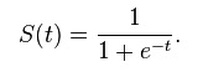
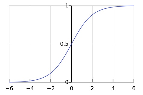
Sigmoid function is a mathematical function having a sigmoid curve. Sigmoid function refers to the special case of the logistic function which is shown in below figure.
(1) Why use sigmoid for MLP
Sigmoid function is a mathematical function having a sigmoid curve. Sigmoid function refers to the special case of the logistic function which is shown in below figure.
|
|
MLP can use activation function of any form, such as logistic sigmoid function of step function. In order to use the back propagation algorithm to learn effectively, the activation function must be differentiable funtion. For this reson, many sigmoid function, especially hyperbolic tangent function and logistic sigmoid function, is adopted as the activation function.
(2) MNIST data set
MNIST is an entry-level computer vision dataset, which contains various handwritten digital pictures. It also contains an image corresponding to each label. and they tells us what is the numbers in the figure. For example, the below four pictures of this label are 5,0,4,1.
(2) MNIST data set
MNIST is an entry-level computer vision dataset, which contains various handwritten digital pictures. It also contains an image corresponding to each label. and they tells us what is the numbers in the figure. For example, the below four pictures of this label are 5,0,4,1.
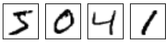
In this example, we will train a machine learning model used to predict the image inside figure. Official website of MNIST dataset is Yann LeCun's website. The download data is divided into two parts: (1) A training data set of 60,000 lines (2) 10,000 lines of test data sets. Such segmentation is very important in the design of machine learning model must have a separate set of test data is not used for training but to evaluate the performance of the model, making it easier to design the model is extended to other datasets.
(3) Backpropagation algorithm
Backpropagation is a common methods used to train artificial neural networks. The method of calculating the network ownership weight loss function gradient calculation. This will be fed back to the gradient optimization method is used to update the weights to minimize the loss function.
The name of the algorithm means that errors can propagate back from the output node to the input node. Back-propagation algorithm can be modified weighting value calculated gradient network errors. This gradient in a simple stochastic gradient descent method is often used to seek to minimize the error weights. Usually "back-propagation" more general use of the word meaning, used to refer to covering the entire process and the calculation of the gradient used in the stochastic gradient descent method. In the back-propagation algorithm suitable for the network, it can usually be quickly converge to a satisfactory minimum.
(4) Gradient descent
Gradient descent is a first-order optimization algorithm. Find a local minimum of a function using the gradient descent, one needs to point at the current step is proportional to the negative gradient of the function. If not, a step gradient being proportional to adopt a local function of close to the maximum; then the process is called gradient ascent.
Learning from group discussion
1. Deep Neural Networks
(1) Except for step function, other activation functions with two properties, such as sigmoid and RELU, and also help neural networks achieve function approximation.
I. The limits s(z) most be well-define as z equal infinity or negative infinity.
II. These limits are different from one another.
(2) There are 6 factors that make the training of DNNs be hard: instability of gradients, the choice of activation function, the way weight are initialized, implementation detail of gradient descent learning, choice of network architecture, and choice of hyper-parameters.
I. Instability of gradients:
The next layer will be faster than last layer, and vanishing gradient occurs, it is difficult to make deep neural network.
II. The choice activation function:
If we use sigmoid function, we may have instability of gradients problem.
III. The way weights are initialized:
If the weights are initialized, there will saturate, and the training will be slow, it is hard to deep neural network.
IV. Choice of hyper-parameters:
Regularization and learning will be slow.
If the learning rate small, the learning will slow.
If the learning rate too large, the learning will be overshoot.
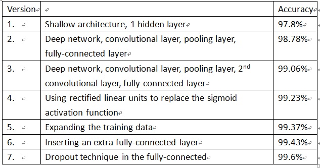
(3) There 7 version of NN/DNN for MNIST with improve accuracy from 97.8% to 99.6%. Each version adds one more technique to the learning algorithm of precious version.
(3) Backpropagation algorithm
Backpropagation is a common methods used to train artificial neural networks. The method of calculating the network ownership weight loss function gradient calculation. This will be fed back to the gradient optimization method is used to update the weights to minimize the loss function.
The name of the algorithm means that errors can propagate back from the output node to the input node. Back-propagation algorithm can be modified weighting value calculated gradient network errors. This gradient in a simple stochastic gradient descent method is often used to seek to minimize the error weights. Usually "back-propagation" more general use of the word meaning, used to refer to covering the entire process and the calculation of the gradient used in the stochastic gradient descent method. In the back-propagation algorithm suitable for the network, it can usually be quickly converge to a satisfactory minimum.
(4) Gradient descent
Gradient descent is a first-order optimization algorithm. Find a local minimum of a function using the gradient descent, one needs to point at the current step is proportional to the negative gradient of the function. If not, a step gradient being proportional to adopt a local function of close to the maximum; then the process is called gradient ascent.
Learning from group discussion
1. Deep Neural Networks
(1) Except for step function, other activation functions with two properties, such as sigmoid and RELU, and also help neural networks achieve function approximation.
I. The limits s(z) most be well-define as z equal infinity or negative infinity.
II. These limits are different from one another.
(2) There are 6 factors that make the training of DNNs be hard: instability of gradients, the choice of activation function, the way weight are initialized, implementation detail of gradient descent learning, choice of network architecture, and choice of hyper-parameters.
I. Instability of gradients:
The next layer will be faster than last layer, and vanishing gradient occurs, it is difficult to make deep neural network.
II. The choice activation function:
If we use sigmoid function, we may have instability of gradients problem.
III. The way weights are initialized:
If the weights are initialized, there will saturate, and the training will be slow, it is hard to deep neural network.
IV. Choice of hyper-parameters:
Regularization and learning will be slow.
If the learning rate small, the learning will slow.
If the learning rate too large, the learning will be overshoot.
(3) There 7 version of NN/DNN for MNIST with improve accuracy from 97.8% to 99.6%. Each version adds one more technique to the learning algorithm of precious version.
2. Neural network
(1) Difference between gradient descent and stochastic gradient descent, and the advantage of SGD over GD. And the relationship between mini-batch and SGD.
(1) Difference between gradient descent and stochastic gradient descent, and the advantage of SGD over GD. And the relationship between mini-batch and SGD.
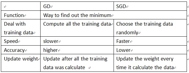
Mini-batch will separate the training data into small group.
SGD with min-batch has both advantage of GD and SGD, it separate the training data into batches and randomly choose one of SGD, for the batch it choose it will calculate the whole data in the batch (GD).
(2) Backpropagation
After we get result, we can compare it with except output.
Then it calculate the cost function, finally it updates the weights layers by layers.
(3) Drop is an effective technique to improve the learning of neural networks and deep neural networks.
All neural will have a chance to been dropout every time it trained, and the neural remaining will this data. Then it recover the network with all the neural. Next time the new data comes, it will dropout some neural again and update the weights.
Conclusion
I am happy for selection pattern recognition course when I prepare this final report. Because when I writing this final report, I know that I really get very knowledge. Teacher and seniors also support me very much so that I think that that is why my English can progress lots of. In this course, I have my first time to take formal English report. Even I still very nervous front of teachers and students, but after this course, I feel that I will have courage to face every report.
